Profiling Kubernetes Applications Using Pixie


In this blog, we will delve into the topic of application profiling and explore one of Pixie’s capabilities: continuous application profiling.
Additionally, we will demonstrate how easy it is to utilize Pixie as an application profiler within a Kubernetes cluster.
Application profilers help us analyze the performance of our application and improve poorly performing sections of the code.
They provide insights into the percentage of CPU usage by various functions in our application, allowing developers to see a comprehensive picture of application code execution and how the resources are being allocated to the application.
Profiling a complex, multi-layered networked application can be a challenging task due to the sheer scale of the application code, chained function calls, and the data structures involved.
Furthermore, as the code base evolves with the addition of new features, modules, and functions, the demand for optimization becomes increasingly pressing.
Using application profilers can provide several key benefits, such as:
- We can make our software development lifecycle more agile.
- Software developers can easily identify the piece of code that has high latency and improve them easily without going through all the code.
- We can enhance the performance of our applications.
As we know, in Kubernetes, our application is running inside a container that is inside a pod. And optimizing the application at runtime will be challenging, as it requires either adding flags to the executing commands or importing profiling libraries into the application code.
It is important to consider both the operating system and our application code’s language when selecting an appropriate application profiler.
This is where pixie comes into play to provide it’s one of the key features of continuous application profiling with no other instrumentation. Pixie installs its agent called Pixie Edge Module (PEM) on each node in your cluster and these PEMs use eBPF to collect data and store the data locally on the node.
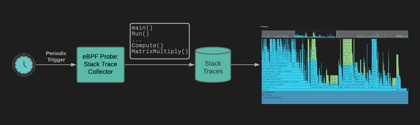
Pixie profiler periodically samples what functions the CPU is executing, and each sample provides a full call stack and we can see all the results in a flamegraph.
Why use Pixie Profiler
Here are some of the reasons why we should use the pixie profiler as an application profiler in our Kubernetes cluster.
-
- It is always running, so we will have real-time application profiling.
- It supports GO, C++, Rust, and Java.
- The sampling frequency is 100 stack trace samples / second / CPU.
- The minimum flamegraph time window is 30 seconds, which can be composed into larger time spans as desired.
- Performance overhead is < 0.5% CPU.
Lets discuss. In how we can use pixie for continuous application profiling.
Working of Pixie’s Application Profiler
Pixie’s continuous profiler uses eBPF to periodically interrupt the CPU. During this process, the eBPF probe inspects the currently running program and collects a stack trace to record where the program was executing. More details on how Pixie uses eBPF are explained here.
Demonstration of Application profiling in Kubernetes cluster using Pixie
We’ve deployed a 3-tier web application on our minikube cluster. We will see the performance of each microservice deployed as a separate pod and see how we can use pixie’s application profiler to monitor the performance of our application.
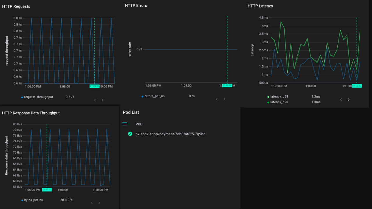
Here in the screenshot above (image B) we can see:
-
- HTTP requests: HTTP requests in a pod.
- HTTP errors: HTTP error counts.
- HTTP latency: Latency in HTTP requests
- CPU utilization: CPU utilization of pod
- Container list: Number of containers running in POD.
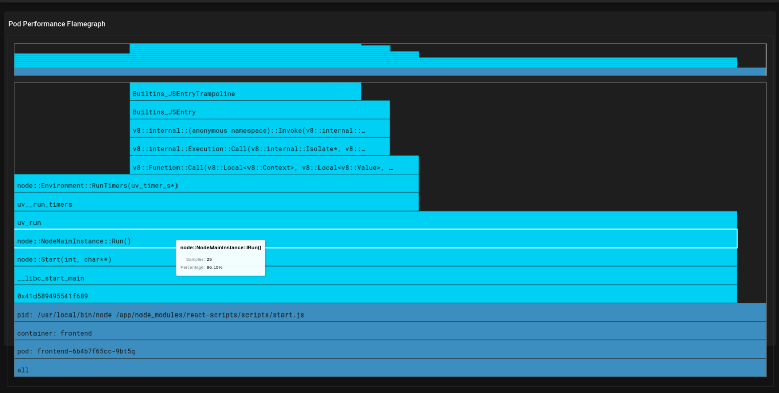
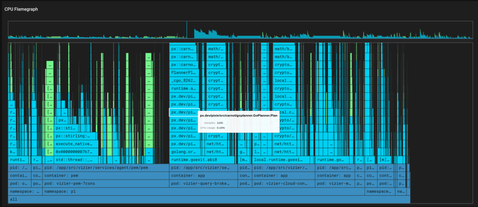
If we want to get the trace of function calls and processes of that application, we can see them in the flamegraph mentioned below.
Every 10 milliseconds, the pixie profiler samples the current stack traces of each CPU, which include the functions that were running at the time of the sample, as well as their parent functions that were called to reach the child functions’ code.
In the above flamegraph (image C), the bars having dark blue color represent Kubernetes metadata and the light blue represents the user’s application code. You can hover over each light blue bar to see the percentage of time of the function’s execution and you can easily see which function is consuming more time and optimize that function’s code.
Let’s take a look at the backend’s pod performance (Image D). In this visualization, the green bars represent the performance of the kernel code, while the light blue bars represent the performance of the user’s application code. By hovering over each light blue bar, it is possible to see the percentage of time that a particular function is executing. This can be useful for identifying which functions are consuming a large amount of time and may benefit from code optimization.
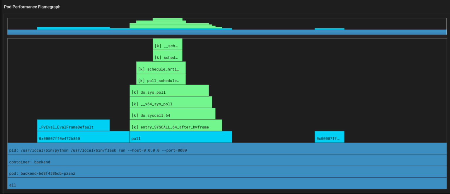
The following flamegraph displays both the applications’ code and the kernel’s code (image E).
Conclusion:
In this blog, we have discussed what application profiling is and why it is important in our Kubernetes cluster. We saw how powerful Pixie is for profiling Kubernetes applications and demonstrated how it can be used to track and optimize application code stacks.
For teams looking to enhance observability and streamline troubleshooting, leveraging Kubernetes consulting services can provide expert guidance on integrating tools like Pixie effectively.
In a future blogs, we will delve deeper into other use cases for Pixie, such as dynamic debugging, database query profiling, request tracing, service performance, etc.
Related Articles

Related Articles
Established in 2012, Xgrid has a history of delivering a wide range of intelligent and secure cloud infrastructure, user interface and user experience solutions. Our strength lies in our team and its ability to deliver end-to-end solutions using cutting edge technologies.
NAVIGATE
Cloud & DevOps Web & Mobile Apps Temporal Digital Marketing GTM Engineering Marketo Consulting HubSpot Consulting Company Careers ResourcesOFFICE ADDRESS
US Address:
Plug and Play Tech Center, 440 N Wolfe Rd, Sunnyvale, CA 94085
Dubai Address:
Dubai Silicon Oasis, DDP, Building A1, Dubai, United Arab Emirates
Pakistan Address:
Xgrid Solutions (Private) Limited, Bldg 96, GCC-11, Civic Center, Gulberg Greens, Islamabad
Xgrid Solutions (Pvt) Ltd, Daftarkhwan (One), Building #254/1, Sector G, Phase 5, DHA, Lahore
Xgrid © 2026. All rights reserved.